TraumaCad Fundamentals

Ian: Okay. So, we’ll make a start. Thank you for joining the session today on TraumaCad Fundamentals. We’re going to cover three areas of TraumaCad. The first one we’re going to start off with planning for an arthroplasty of the hip. We’re then going to go ahead and do the same for the knee. We’re then going to do a case looking at a deformity correction. After that, we’ll have a question and answer session. So, that will be the section where you can ask questions on any of these subjects. But to keep it focused, we’ll spend 15 minutes on each section. So, we’ll spent 15 minutes on hip. If you have any burning questions that you’d like to ask related to the planning of the hip, you can ask that at the end of the hip session. But if you find that there’s a question that’s really burning, feel free to ask that in the chat. My colleague will be keeping an eye on the chat and we’ll make sure that we answer your question as we go along. But if you could keep yourself muted because there’s a lot of people on this webinar. So, we want to make sure it flows smoothly. So, if you do have a question, if you could ask that question in the chat.

Okay. So, TraumaCad. TraumaCad is a software that has been in the market for about 10 years. It’s a product, it’s a solution offered by Brainlab. Okay. So, let’s go ahead and go straight into TraumaCad. Right. So, the first screen you can see is the screen that you will typically see in TraumaCad when you launch TraumaCad from your PAC System. We can connect to any PAC System. So, once you’re in the PAC… When you’re in the PAC System to access TraumaCad, if you are looking at the pelvic image, you just have to click on a button within the PACs and typically that will launch the image that you were looking at directly into TraumaCad. So, you don’t have to log out and log in again. The image will be pulled directly from your PAC System.

The image is populated in the top-left-hand side of the screen and you’ll see the patient’s first name, last name, the patient ID, and the accession number. You left-click on that image, and then you can choose the procedure. As you can see, there’s a number of procedures within TraumaCad. You can use choose to plan a hip, a primary hip arthroplasty, or a revision, or a Hemi. We can plan for knee, including unicon diagnose, primary knees, revisions, or prelim shoulders, including reverse shoulders, foot, and ankle. There’s a lot of tools within TraumaCad, for instance, hindfoot osteotomies, pediatric. There’s a whole section on pediatrics, a section on deformity correction including high-tibial osteotomies and distal-femoral osteotomy or complex deformity correction, which we’ll be looking at later on in the presentation. Trauma. There’s a lot of things you can plan for trauma. And there’s some spinal tools as well, for instance, looking at call bangles or pelvic radius angles or other data areas within a spinal orthopedics.

So, let’s go to hip. I’m going to left-click on the hip icon. The first thing the software does, it looks for a calibration device. The calibration device can be a single calibration ball or as you can see on this image, it’s the KingMark. So, the KingMark is a device that makes calibrating for an AP pelvis very accurate. The software has found the KingMark, so now we will identify the projection. So, it’s at AP view of the pelvis. And we’ll select the site that we want to plan. When I do that, I can press Accept. And if you notice in the bottom corner of the screen, when I press Accept TraumaCad is going to calibrate this image. So, there we go. And for this particular patient, it said the radiographic magnification is 13%. And as you know, you would expect that figure to be anywhere from 10% to 30%, but the average will be around 15% or 20%.

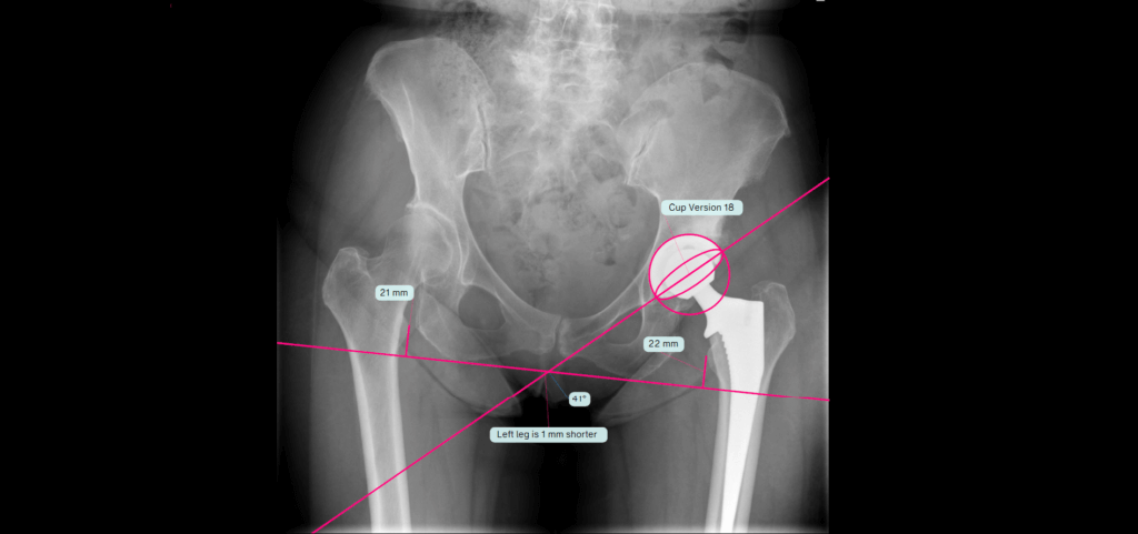
Okay. So, we can now confidently know that when we measure anything on this image, it is life-size. So, let’s choose the manufacturer. Now as you know, there’s many manufacturers in orthopedics. So, we have the whole library over here. So, we can select the manufacturer that you want. So, let’s take Smith and Nephew. You can start with the acetabular component, the cup, or if you’re working practice you prefer to start with the stem, you can start with the stem as well. So, let’s stay on the cup, and let’s choose the cup that you want. So, let’s take an R3 cup. I’ll double-click my mouse on the R3. And you’ll notice the behavior of TraumaCad. It’s placed the cup roughly into the right position. We never suggest a position. We just put it somewhere near. The software also did a leg length discrepancy, referencing off the transition line and the midpoint of the lesser trochanter. So, we can look at that and you can see that TraumaCad using AI and various other algorithms has actually identified that automatically for you. The important figure, of course, being the difference between the left and the right leg. So, TraumaCad is telling you that there’s a four-millimeter difference.

The software has also placed the cup in a reasonable position at a radiographic inclination of 45 degrees. If you prefer a different inclination, you can hold your mouse on the yellow button and change the inclination to what you’d like to use. So, when we’re happy with that, we can then…to move the cup, you can hold your mouse within the yellow border and drag and drop the cup to wherever you’d like. You can magnify the image purely by using your scroll button between your left and right-hand mouse. So, we can position the acetabular component and you’ll notice there’s some osteophytes in this patient. So, we can ignore the osteophytes and we can change the size to what we feel is right for this patient. Once we’ve done that, if you prefer to use the teardrop as your landmark, we can drag the line, grab the line here, and move on to the teardrop. So, TraumaCad allows you the flexibility to use the workflow that you’re familiar with. If you do make a mistake, it’s very easy. All you have to do is use the undo button and it will sequentially undo every single step you take. And you can read through every single step as well.

Okay. So, we’ve planned our acetabular component. We can now add the stem. So, we go to Templates, and we can then add a template. And we can change the definition to Stems. And we can choose the stem that we want. So, let’s say for us that this one would take a POLARSTEM Non-Cemented. Once again, you notice the behavior of TraumaCad. It’s placed the stem roughly into the right position. All you have to do now will magnify the image and we can move the stem to where we like. We can then change the size of the stem as well. And we can get a very good feel what would be the correct size for that particular patient. Okay.

The fourth thing TraumaCad is it threw in a generic resection line. So, you can move your mouse on to the generic resection line and you can match it to where you’re going to do your cut. So, this gives us some valuable information. We also know over here the distance between the center of the cup and this attachment point on the stem is nine millimeters. We also note that the vertical distance between those two points is six millimeters. So, essentially what we want to know next is what happens to the leg length when we attach those two points. So, we’ll right-click on the stem. We’ll left-click on attach to stem and it attaches the two points. So, you can very clearly see with your components positioned in those positions what effect this is going to have on the patient. So, we’ve corrected the limb length discrepancy by two millimeters. Obviously, the offset between those two points was nine millimeters, so we’ve affected the offset by nine millimeters.

If, for example, you weren’t happy with that and you wanted to try a lateralized stem, you can click on the lateralized stem. If you say, «Well, I’ll stay with the standard, but I want to see what happens if I use a longer neck or a longer neck or maybe a shorter neck.» Supposing your entry or preoperative landmark is the distance between your resection line and the upper limit of the lesser trochanter. We will magnify the image. We’ll take the ruler from the toolbar and we can measure that. So, we know preoperatively our resection line is 15 millimeters above the upper limit of the lesser trochanter and this is what we can then use as our landmark intraoperatively. If for a sake of argument you were doing an anterior minimally invasive approach, we can always measure from the greater trochanter to the shoulder of the stem.

Let’s say we’ve now finished the plan and you want to save your planned image back into the PAC System. How do we do that? We go to the Report tab, we save the case, we can also produce a report. But if you want to save the case, we can go straight to Save Case. That box will be ticked already. You just press OK and it sends that case back into the PAC System underneath the patient saved accession number. It’s important to point out that we’ve copied the original DICOM image and we’re sending the copy back to the PAC System. So, we never affect the original image. When you’re in the operating room now, both the patient’s image pre-planned and planned can be brought up on the screen, and so you will have a good idea and the operating staff can have a good idea what you want and what you’ve planned. Obviously, we can’t be 100% right all of the time. But provided the preoperative X-ray is of a good quality and has a calibration device on the image, it’s highly likely that the component you’ve chosen will be the same size that you actually insert or it may be one size either side, typically. So, you can see that this can very much positively affect the workflow.

Let’s cancel that. So, we will pretend we’re not sending it to the PACs. And we say we finish this case and we do the next case. Now, I want to show you an even faster workflow. And you know it’s not all about speed. It’s also done to accuracy. So, let’s choose a different case and we’ll say this is the next patient. We’ll go to hip. The image is calibrated when I press that and we say we’re doing a right hip on this occasion. I’ll press Accept. You can, of course, go back to recently used. As opposed to looking through the whole list, you can go to recently used and that automatically gives you your list what you use most commonly. But we can also go to Kits. You can create kits for whatever you like. We can double-click on that. And you’ll notice that it put the acetabular component and the stem onto the image with one click. You can then adjust the position of your components, adjust the size of your component. And then when you’re ready, we can put the resection line to match the actual resection point. And once we’ve done that, we can then do Attach Stem to Cup as we did before. And it does that.

Okay. That’s the first section, planning a hip. We’ll now go on to planning a knee. If there’s any burning questions on the hip, you can now say none or you can save it to the end of the session. So, we’ll go straight on to that knee. So, let’s select a knee. The behavior is exactly the same as I showed for the hip. So, we’re launching the images or the image directly from the PAC System. We’ll now choose the views that we want to plan. And we’ll press Next. We can now go on to the knee icon. Once again, the behavior is the same as previously. If there is a calibration ball on the image, the software finds it automatically. So, we’ll identify the view and the leg that we’re going to…the knee that we’re going to plan for. And then we’ll press Accept. The software then finds the calibration ball on the lateral view.

So we can just identify that and except. We’ve got a culminated view of the knee. But to show you that there’s actually the ability to plan on a full-length image as well, weight-bearing, we can do certain tools. There are tools in there for outcomes. If you’ve already implanted the knee and say, for instance, the following year or the year after that you want to assess if there’s been any subsidence of the implant. You can do that within TraumaCad as well. Some surgeons as we know would prefer just to go straight to the templates and choose the template that they want. But it does give you the ability to actually look at mechanical and anatomical access as well. Bearing in mind that this is a culminated view of the knee, so we can’t see the center of rotation of the femoral head or the ankle, so that the gold standard would be a full-length view. But I just want to show you what’s most commonly the images that are most commonly in use in the vast majority of radiographic departments.

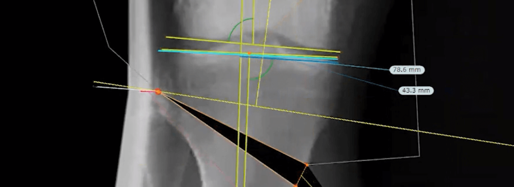
So, with the culminated view, we can still get some very useful information. So, the first line says AP Resection Line. Let’s just click on that. And it puts those lines on to the image for you. So, it’s identified the anatomical access through the tibia, the anatomical axis through the femur, but it’s also extrapolated a dotted line to the average center of rotation. Now, of course, we can’t see the femoral head. And if you feel that the mechanical axis for this patient is near four degrees, you can drag that across to emulate that. Let’s just magnify this AP view. So, what we’ll do, we’ll double click and we can magnify it and we can look at these lines. The software has automatically identified the contours of the femur and on the tibial plateau. So, we can now adjust this to see what the effect would be depending on how much bone we want to resect. And it shows you what… If we looking at the medial condyle of the femur, it will then say if you’re resecting 10 millimeters to maintain the access, you would need to remove 6 millimeters on the lateral aspect. And the same follows for the tibia.

So, when you’re happy with the amount of bone you’re going to resect, we can then start to look at the implants. So, we’ll go back to the templates now. And we can look at the various implants that are available. And as you can see, once again, the library is very extensive. So, let’s take a different manufacturer. Let’s just go for Depuy. And if you want to start with the femoral component, we can change that. And you can choose the actual model that you’d like. So, let’s go for the Attune. We double-click on the Attune. And you’ll notice the software on the AP view has matched the component to the resection line. On the lateral view, we just moved back manually into the ideal position. And one of the things that obviously we’re very keen to see is the component size.

So, we can look at different sizes. We can click on different sizes to get the idea for this particular patient. So, when you’re happy with that, we can then go ahead and choose the tibial component. So, we change this from Femoral to Tibial. And we can choose the implant that we’d like to use. So, let’s just say we’ll use a for instance, the rotating… Sorry. We didn’t want the insert. Let’s just go back a step. This shows you that if you do make a mistake, you can go back. So, let’s go for the attune and let’s go for the rotating platform over here or we can go for this. So, it really does give you some great choice of what components you want to use. So, let’s adjust it on the lateral view. And we can look for the correct size. And on the AP view, we can do the same. So, let’s just look at the different sizing over here. And then when you want to look with the components in that position, we’ve got some valuable information about the actual axis as well whether it’s virus or valgus. And we can also look at the limb alignment. When those two cube components are implanted, we can then look at that. We can show alignment and show what the final alignment looks like.

So, once again, you can see that it’s logical steps to navigate through TraumaCad. When you finish, you can go to Report. And once again, we can show the report which I didn’t do on the hip, but we can show it and this would be the same for the hip as well. So, we produce a report that also goes back to the PAC System. So, you can see the size you’re using, the model number, the part. We can even input the surgery institute and the date that the surgery is planned for. So, once we’re ready, we can go to Report and save the case, and that saves it back into the PAC System. So, you can see that the workflow is very similar. But let’s say we are on the next patient. Let’s go to the next patient because we can do the same as we did with the hip.

So, let’s just launch this. For sake of privacy, we’ll use the same patient. But let’s just say that this patient was the next patient to attend and we wanted to do some planning. So, let’s say identify the AP view and the left lateral view. We’ll accept. So, similar to what we did before, we can do a drop in the resection lines. We can go to Template, and we can go straight to Kits. I can double click on Kits, and that drops the implant in for us. We can fine-tune the positioning of that. And then we can look at the final alignment, and we’re finished. So, you can see, once again, to emphasize the steps are very straightforward.

Okay. So, it looks like we’re running absolutely fine timewise. We’ve actually got slightly more time. And in fact, that’s a very good thing to have because we’re going to not look at a complex deformity correction. So, let’s say we finished with this patient. We’ll now go to a new case. We’ll say OK. And we’ll choose a deformity correction case. So, let’s just choose a case that has got a very exaggerated bilateral virus. So, we choose this case here. And we’ll launch the image. This time we’ll go to deformity correction. Once again, if there’s a calibration ball and the ideal for a full-length weight-bearing image would be a calibration ball just lateral to the femoral conduct of the affected side. If that’s the case, the software would have found that automatically as per the previous images we were looking at for the knee. In this case, there’s a ruler in the midline.

So, we can use the ruler as well. Your radiographers don’t have to change their practice. They can carry on and use the ruler. So, let’s identify the image. We’re going to concentrate on the right sight, and then we can manually have a look at that ruler and calibrate it. Now, obviously, that’s really small. So, we can magnify the image. And we know that from 80 to 90, it’s 100 millimeters. And then we can Accept. And we’re now working on a calibrated view. So, let’s Fit to Screen. And you’ll notice there are various tools on the left-hand side under measurement tools. So, the one we’re interested is Limb Alignment. You can choose to do a Unilateral or you can do a Bilateral. It’s advisable to do a Bilateral because, obviously, we’re going to glean more information as regards the comparison between the left and right leg. So, let’s choose Bilateral.

And then you can use a magnifying glass if you prefer, but you don’t have to. And then you have the ability to choose… Sorry. To select the various landmarks on the image. So, we have a little guide on the left-hand side of the screen that’s guiding me where to put the marker. So, let’s mark the center of the right femoral head. The next marker is asking me to mark the tip of the greater trochanter on the right. The next marker is asking me to put that at the most convicts point on the right medial femoral condo. Now, I’m not going to read these out because now you’ve got an idea where I’m placing these landmarks. So, all I’m doing is simply following the diagram on the left-hand side of the screen. If you make a mistake, the best thing to do is put the markers on first and at the end, we’ll fine-tune. This is actually version 2.5 of TraumaCad. In the next version, it’ll be one click and the software will put all of these markers on for you with one click.

Okay. When we put the last marker on, we get some useful information on the top-left of the screen. But before we do anything, you’ll notice that I put those markers on very quickly. So, now is where we’ll fine-tune. So, we’ll go to the knee on the right side. As I said, we’re just going to concentrate on the right side. I’m aware there’s growth plates here, so we wouldn’t necessarily be doing an osteotomy on an adolescent. Let’s just add this particular adolescent, actually. So, let’s just use that. Now, we could go most concave on the tibial plateau, but as you know, if the X-ray wasn’t taken with exactly or very close to 90 degrees to the knee joint, then it’s sometimes difficult to differentiate the posterior tibial plateau to the anterior. So, in this case, you could actually just go for the outer limit on the medial and the lateral tibial plateau.

So, once we’ve done that, we can now go to the plafond and we can correct that. So, we can see what it looks like. And you’ll notice that if it’s within the normal range, if you refer to the top-left-hand side of the screen, if it’s within the normal range and the normal range is identified for you over here, then the actual figure is in green. So, we can see that the mechanical lateral distal tibial angle is 90 degrees, so we’re not concerned that the ankle looks fine as regards the weight-bearing axis. We can do the same on the left-hand side. And we can then go to the central to femoral head and we can say that’s all fine. So, now you can see immediately something is being made aware to us that actually the virus is not only in the tibia, but there’s actually a subtle deformity in the distal femur.

So, let’s start off by doing one osteotomy. If we start drawing in lines and we start looking for CORA, there’s going to be a lot of lines on the image. Yes, we are interested in the analysis, but what we want to do while we’re looking to identify the CORA is switch that off. So, it’s important to point out that we’re not deleting the limb alignment. We’re actually just hiding it. Now we can start to look for CORA. So, as I said, we’re going to look at the CORA for the proximal tibia. So, we have a nice diagram on the left where you can choose the appropriate lines that you want to use to identify CORA. So, let’s use the proximal tibial joint line. And let’s use a centerline find on the tibia to identify the anatomical axis.

So, we can very accurately by enlarging the image be very accurate in identifying the outer cortex. Now, you’ll notice that where the two lines intersect, we’ve identified the CORA. Let’s look at the CORA. So, we can see the orange knot in the middle is the CORA, but the software has also drawn in a generic resection line for you. There’s also the bisector line if you’re using an external fixator. But let’s say we’re going to do the osteotomy at this level. And we’ve identified the hinge which is represented by this red circle. If we chose to do a closing wedge osteotomy, we can simply click on Close and it puts the hinge on the opposite side. Now, obviously, that’s not relevant for this patient, so we’d leave it as an opening wedge.

We’ll now Fit to Screen. We finished with the CORA lines. So, they’ve served their purpose. So, we can now switch them off. And once again, we’re not deleting lines with simply hiding them. So, what information have we got now? We’re going to switch the Limb Alignment Analysis back on. And we can see that our MAX, Mechanical Axis Deviation, is very medial. So, we want to now assess how much to open up the wedge once we’ve done our osteotomy to get the mechanical, the weight-bearing axis in a more acceptable plane. So, let’s finish and cut. When you finish and cut, this forms two components. So, we’ve got the proximal component here and we’ve got the distal component articulating around the CORA. When I click on the distal component, I’ll magnify the image at this stage so that we can see it clearly. So, we want to start opening up the wedge now to see how much we have to open up that wedge to actually get the mechanical axis, the weight-bearing axis in the appropriate position. Now you can see, as I’m moving up that wedge, we’re going too far because our mechanical axis is still not. If you refer it to Fujisawa, then you know that your mechanical axis is still too medial.

Let’s see what happens if we do take it to 50% or 55%. You can see, yes, we’ve corrected the axis, but we’ve taken an impossibly large wage. So, you know that this is going to overstretch the public [inaudible 00:29:59] the nerves and so we can’t possibly do that. So, how are we going to correct for this patient? We can say, «Okay. That’s unacceptable wage. So, how are we going to get our mechanical axis correct?» This is a patient or this is a case where we may choose to do a double osteotomy.» So, how are we going to do that? We’ll Fit to Screen so that we can see the whole length. We’ll undo the cut. And now we can look for a second CORA. So, same as before, we’re going to hide the limb alignment analysis. We’re going to go to the box at the bottom of the screen to add a CORA. You’ll notice now that we’ve got two tabs. So, we’ve got CORA 1 and CORA 2. And if this is a highly complex case, you can actually select four CORA on the same site.

So, let’s go to the distal femur now. And we can choose a mechanical or an anatomical femoral joint line. It’s important if you do choose an anatomical that the second line is also anatomical. If you choose mechanical, then you have to make sure that the second line is mechanical. So, let’s stay with anatomical. And we’ll select that and it’s placed the line for us on the femur. Let’s bring our most medially and select the femoral centerline finder. So, similar to what we did on the tibia, we’re going to do the same on the femur. So, we’ll magnify the image so as we can see it clearly. We will then identify the outer cortex and we’ll put… We’ll identify that and put a marker on the outer cortex so we can read really accurate here. Let’s do the same distally. So, we’ll identify the outer cortex and medially as well. So, we’ve got a very nice line through the anatomical axis of the femur. Let’s Fit to Screen so that we can see the whole length. And now we’ve identified two CORA, but we’ve got a lot of lines on the image, which is going to confuse us when we start looking at the axis. So, once again, let’s hide those lines by switching the box off.

Okay. So, we’ve identified a second CORA at the distal femur. Let’s magnify the image so as we can see it clearly. We know that we don’t want to do our osteotomy that close to the knee joint. So, we can move our osteotomy line approximately and we can choose where we want to do the hinge. So, we can take that. And if you wanted to measure up from the knee joint, you can take your ruler and, say, for instance, you want to do your osteotomy at eight centimeters or five or whatever from the knee joint, you can be very accurate with that. So, let’s just say we’re doing this at six centimeters. Okay. Let’s get rid of the ruler because we’ve used it now. We’ve got enough lines. We don’t want another line to confuse us. So, let’s delete it.

Now, at present, we’re set for an opening wage on the femur and we don’t want to do an opening wedge. So, we switch to a closing wedge. So, our hinge is now on the medial aspect. Now bear in mind, we’re doing an osteotomy distant from the CORA. So, we’re also aware that we’re going to get translation. So, let’s now Fit to Screen. And we’ll switch a limb alignment lines back on. We can now finish and cut. And we can auto-align. Now watch over here because we want to know what happens on the left-hand side to the mechanical axis when we align the two components. Sorry. The two lines. So, we’ll auto-align. And that’s what it does. So, you can see that we’ve corrected. Everything is now looking correct. We can also see what effect that have on the overall length on the right-hand side. So, we’ve actually lengthened by about eight millimeters on the right-hand side.

So, let’s have a look more closely at this. We’ve said we have got a bit of translation there, but let’s just correct that. We know that if we open up a wage of 8 millimeters, 10 degrees… Sorry. Close a wedge of 8 millimeters and 10 degrees on the distal femur and we open up a wedge of 10 millimeters and 16 degrees, then our mechanical axis, our weight-bearing axis is such. If we decide that we’re not happy with that and we want to move our weight-bearing axis more laterally, we can say we’ll close the wage slightly more. Or if you want, you can leave it there and say, «Well, what happens? I also have the option to open up this wage more as well.» So, you can see that the software is very flexible. It’s able to give you a lot of valuable information prior to taking this patient to the operating room.

Now, supposing you were in a training environment and you wanted to show the trainees additional to do in the osteotomy, which manufacturer which template which plate you want to use, or if this was a case where you were doing a destruction, we can also have the nails in situ. We can place the nails in situ and we can actually represent the destruction. But let’s say, for instance, just to show you, we have the templates within TraumaCad, so we can select that. We can select the manufacturer. So, let’s say, for instance, we may want to see a synthes plate, we can choose that. And if you want the tibial effects, that’s all in there as well. But equally. So, if it’s a new clip or if it’s a fit bone or if it’s an orthopediatric case, we have a very extensive library. So, it’s not matched to one manufacturer. It’s agnostic. So, we have all of the manufacturers in the software.

Okay. So, we finished now. We can go to Report and we can see that we want to save this case back into the PAC System. So, we’ve showed the report. And once again, this has some valuable information for you. And in some centers, this is actually used as the patient information tool. So, you can actually show your patient and say, «Look, this is what your present situation is and this is what the surgery is going to achieve for you.» And actually, this is a very useful tool because you know that if you say to a layperson that you’re going to cut their femur, basically, you’re going to break it and you’re going to cut their tibia and move it around, they may be quite horrified hoping they can see what you’re doing that for and what you’re aiming to achieve it’s a lot more acceptable. Okay. Great. So, we finished. We’ve gone through, once again, a hip case, a knee case, and a deformity case. So, now we’ll open up the floor for any questions and answers.

Chen: We have a question in the chat from Thomas D.

Ian: Okay.

Chen: And he asks if it’s possible to have frontal and sagittal view for hip cases or only frontal view.

Ian: Yeah. So, if the question is related to a lateral view and an AP view or a turned view or for the lateral instead of a lateral view, absolutely. As you know, with the hip case, we may well be looking at femoral impingement. So, it just so happens that just… I don’t actually have a lateral view on this particular case, but you’re absolutely correct. If there was a lateral view below here, we could launch both views and then we can actually plan in both views to look at the femoral impingement or the alpha angle so we can do that as well.

Chen: And the next question is, how would you plan a dysplastic hip where anatomy is not so well defined as in the case you demonstrated?

Ian: Yep.

Chen: You used the 3D CD model.

Ian: Yeah. That’s a very good question. So, let’s go to a case and let’s just use a case where we may want to do some more analysis around the pelvis. So, let’s go to this case. I’ll just pick any case. This obviously is a normal case, but it may well not be. In fact, I’ll just take the case below it. We’ll use the same case we used before. So, now, let’s launch and we’re going to hip. The software thinks that we want to do an arthroplasty, but let’s say, actually, we don’t want to do that at this stage. We want to look at the dysplastic hip or some other form of severe osteoarthritis, whatever the pathology is that’s presenting. So, rather than going to templates, we’ll switch across to measurement tools. So, we have a number of different tools you can use. So, let’s say, for instance, we want to look at the hip outcome preoperatively or postoperatively, or let’s do a hip deformity analysis.

Similar to when we were doing the deformity correction, I’m going to switch the magnifying glass off. The reason I’m doing that is because if it’s a very low-contrast image, you can see that the magnifying glass is actually not very helpful. If this was a high-contrast image, then maybe you would be able to glean more information using the magnifying glass. So, let’s switch that off. And once again, you have a diagram on the left-hand side of the screen where we can choose the relevant landmarks. So, let’s mark the first landmark on the super lateral edge of the right-hand turbulent, then on the left, then on the teardrop, and on the left. And once again, as we did with the deformity case, I’m not going to read all of these out. You can see. You get the feel of what I’m doing. So, I’m just following this diagram with the instructions where to put the markers.

Okay. I wanna put the markers on. Same as before, we can fine-tune so that we’re happy with those markers. And then we can look at central edge, reimer index. So, there’s lots of different things you can do. And just supposing this as a note as we pointed out, this is a normal case. But let’s say, for instance, you were doing an osteotomy. So, let’s define a fragment. You can click around, whatever you like. And you can put these markers as close together or as far apart as you’d like. Okay. Just say for sake of argument, we’re doing an osteotomy here. The software has identified that fragment for you and it’s created a center of rotation. Now, you may say that’s not the center of rotation I want. I want to put it on the center of the femoral head. And as I said before, we can fine-tune these. So, we can make it look nicer. That’s not essential, but it kind of looks a bit nicer when we start moving things around.

Okay. Let’s say we’re doing an osteotomy here as an example. So, there’s the center of rotation. And we can now move that. And watch what happens here when we start moving now. Okay. Nothing’s changed at present because that’s normal, but if it was these would change over here. Let’s say, for instance, we’ve done an osteotomy and we’ve moved into that area. Let’s Fit to Screen and let’s create a second fragment. Okay. So, we can now move that there. And we can get a very good feel of what we’re trying to do and how it’s affecting the parameters here with a dysplastic hip tried to correct it for that particular patient. As you know, radiographers, and this applies to lots of different countries, they go through quite an extensive training.

And part of their training is to identify the most appropriate accurate view prior to surgery. So, as an example, if we go back into the same case, the radiographic parameters for an AP pelvis prior to hip surgery or even in any other case is to take a view without rotation of the pelvis in relation to the X-ray table or the trolley with the legs internally rotated by 15 degrees. Now, why is that the case? Because in that view, you get the correct plans of the femoral neck. So, if that leg was externally rotated, you would get a good indication of that because the lesser trochanter wouldn’t be in the correct plane. If it was internally rotated too much, the same effect would happen. You would see less or more of the lesser trochanter.

So, an answer to your question, there is no guide within TraumaCad because the understanding is that the radiographers in conjunction with the orthopedic department have worked out the protocol that is relevant for the particular case. Now, as I said, the standard projection is a low-centered AP pelvis if it’s a case going for a total hip arthroplasty with the legs internally rotated 15 degrees. And of course, the parameters are different for different parts of the body. If this was a case, that was a deformity correction. The important… One of the most important things is that there’s an extended film focus distance.

So, the X-ray tube is typically placed at a full-film focal distance of 1.8 to 2 meters. The patient is standing with ideally the calibration ball placed mid-point from AP to leg… Sorry. From posterior to anterior at the level of the femoral condo. Yes, it could be placed further down the leg, but with a diverging X-ray beam, it’s better to have it at 90 degrees to the X-ray beam. Also, in that case, once again, this goes back to radiographic practice. If there is a pre-existing leg length discrepancy, then blocks of the relevant size are placed under the affected leg so that you can get a true idea or understanding of where the deformity is arising from.

Chen: Great. We have another question here from the audience. How do you make sure that the X-ray is calibrated for a hip?

Ian: Okay. Once again, a really good question because you’re absolutely correct. In the ideal world, it would be great if every single patient coming through for a total hip arthroplasty has some form of calibration device on the image. But as you know, that is not always the case. So, say, for instance, we ignore the KingMark on this image. And we’ll pretend because I actually haven’t gotten an image without the calibration ball. In fact, we’ll use a different image. Let’s say we’re going to use this image because I think the audience may be used to seeing a single calibration ball. So, you can see that the software found that automatically. But let’s pretend that that calibration ball was not on the image. How would we calibrate that image so that we can carry on and plan the case for this patient? What we’ll do, we’ll say… We’ll identify the projection. We’ll identify the site. And as you can see, there’s a lot of osteophytes on this patient. So, probably, a very good case to be able to plan preoperatively. But we’re pretending that the calibration ball is not on this image.

So, in this case, we can go to the Oversize button. We can select that. And earlier on in the talk, you may remember that we said the average magnification for an adult’s AP pelvis is approximately between 15% and 20%. The additional information that you as a surgeon would have not just the X-ray in front of you, but you also have the benefit of having the patient, not necessarily in front of you at that time, but during the clinical workup you’ll have seen the patient. So, if the patient is very slim, it would be a fair deduction that the magnification factor would be less. So, you may allow 10% magnification in that case. If it’s a large patient, and even if you hadn’t seen that patient, you can tell from the X-rays, the amount of adipose tissue. So, you could glean from that that this is a larger patient. So, you may allow 25% or even 30% magnification.

But we know that this is an average-size patient. So, we’re going to go to the Oversize button and we’re going to type in 120%. We’ll now Accept. And in the bottom side right-hand side of the screen, you can see that we’ve allowed 20% magnification factor for this patient. If retrospectively you find that that was incorrect because you planned a size 6’10 and you actually implanted a size 8, then you can retrospectively go back not for that patient, of course, to plan it, but you know that the next patient that comes through your department, the average magnification is around 15%. Yes, this is a workaround. The ideal situation is if the radiographers can be trained to actually place a calibration device at the appropriate level from the X-ray table.

Chen: Great. We have another question. Do you have a 3D solution for hip planification?

Ian: That’s a very good question, once again. As we go… As the market evolves, we find particularly in the European market that not for every case, but for more complex cases, 3D does add value preoperatively. There’s no question about that. To go into a little bit of the history of Brainlab, we are very skilled in intraoperative navigation. In fact, the name comes from the very birth of Brainlab because it was actually born around intraoperative neuronavigation where the founder of the company, Stefan Vilsmeier, worked with neurosurgeons at AKH, the University Hospital of Vienna, to develop stereotactic intraoperative navigation. What about 3D planning preoperatively? Where that is the case, we have something like 300 up developers more than in Munich at our headquarters who work on very sophisticated rendering for 3D. So, that’s why I say we know that it adds value.

From a Cad, the development team that work with TraumaCad also work with AI and big data. So, we took a conscious decision not to develop 3D preoperative templating within TraumaCad, but to choose the market leader, which is LEXI, which is a Japanese company that has hundreds of installations in Japan and have been in the market and have a lot of experience with 3D planning. The European office has opened up in Germany. So, we work in partnership with LEXI. So, we’ve taken the best of breed and partnered. So, yes, we do have a 3D solution in the guise of LEXI. And you can plan hips in 3D in conjunction with your 2D planning with TraumaCad and 3D using our partner’s 3D solution.

Chen: Great. We have one more question. In the planning for revision hip or knee, does TraumaCad could allow identification of primary implants and removal of the implant on the image to allow assessments of bone defects?

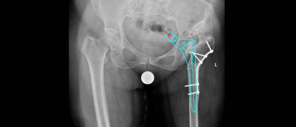
Ian: Once again, that’s an excellent question. There’s a number of things we’re doing around gleaning more information for revisions because we all know that this is an area which is becoming much more critical for patients. So, let’s, as an example, go into a case that may be true for revision. So, let’s launch the image and let’s calibrate the image. And then we want to do some analysis around this stem to see what the bone structure would look like during this revision, bone stock, and also to look at the mechanics, the biomechanics of this joint. So, let’s have a look at some measurement tools. So, let’s go in. And you may remember that we were scrolling on this list and looking at various tools.

As an example, let’s just say we were looking…we wanted to do some outcome postoperatively. So, this could be in a center where there’s a lot of analysis happening postoperatively and you know that that can be quite time-consuming. Okay. So, let’s just go into Post Op. Once again, we’re following the same pattern as we did before. So, we’re identifying landmarks. So, we’ll identify the teardrop. Yes, there’s a lot of cement on the right-hand side. But let’s evaluate where the teardrop is. We go to the midpoint of the lesser trochanter. We go over here on the shoulder. We’ll go midline. We’ll then go to the cup here. Once again, I’m not going to read all of these out because it’s quite… You can see what I’m actually doing.

Okay. So, I know that I haven’t fully answered your question. So, what can we do in addition to this information that we can glean prior to doing the revision? Well, we’ve got the center of rotation. We know what the medial offset looks like now, we know what the hip height looks like, and we know what the alignment is, varus or valgus. Over and above this, there are certain things that I can’t mention in this call. But we are working with a group of surgeons who are looking and are looking at many, many thousands of post-operative cases to not only for hip arthroplasty revisions, but also for trauma, to be able to identify from the image what implant had been implanted 10, 15 years ago. To automatically identify that implant, as you know with trauma, when you’re looking at these kits for removal or also with hip arthroplasty leading to a revision, it would be very useful to know which implant is implanted so that we can work out the plan for that patient when you’re going to do the revision. Now, I’m not pretending we have that in TraumaCad yet, but as I said before, we have a very big development team within Brainlab and it’s something that we look to external experts who can then input that data that may affect the development of the software.

Just before we finish, I’d like to share one more thing with you. Obviously, that training session has gone through fairly quickly with the fundamentals. But as we say here, yes, we’re a high-tech company, so we can use social media. So, let’s keep in touch. Feel free to reach out with us. We have many very valuable teaching videos on YouTube. We have Facebook. We have a TraumaCad page and group within LinkedIn and, of course, Instagram. So, we encourage you to keep in touch with us. If you have any questions that have arisen from this presentation, please do let us know and we’d be very happy to align with you, and if required, even set up specific webinars for you or a web call with you individually to go over the software. We’re very keen that with our software users are familiar or can get familiar with the software. And that’s what we’re there for. And I think that’s it. I think we finished the webinar. So, once again, thank you all for attending.